
Introduction
Median is a useful statistical function, which first time appeared in SSAS 2016 and in Power BI around that year as well. There are several articles on how to implement the median function in DAX from the time before the native DAX function was introduced. With one client we recently faced an issue when using the implicit median function in Power BI. Size of the dataset was roughly 30mio records. I would say nothing challenging for Power BI or DAX itself. However, the behavior of the median function was not convincing at all. Let’s look at the setup:
I created a median dataset based on free data from weather sensors in one city (a link to download at the end of the blog) which has similar data characteristics as our report with the original issue.
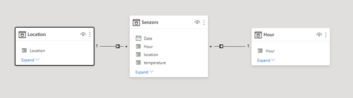
We have the following attributes: date, hour, location (just numeric ID of location which is fine for our test) and we are monitoring the temperature.
We have 35mio records -> 944 unique records for temperature, 422 unique locations, and 24 hours of course. 🙂
Now we make a simple report – we would like to see the median for temperature per hour despite date or location.
Measure:
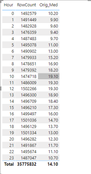
| MEASURE Senzors[Orig_Med] = MEDIAN ( Senzors[temperature] ) |
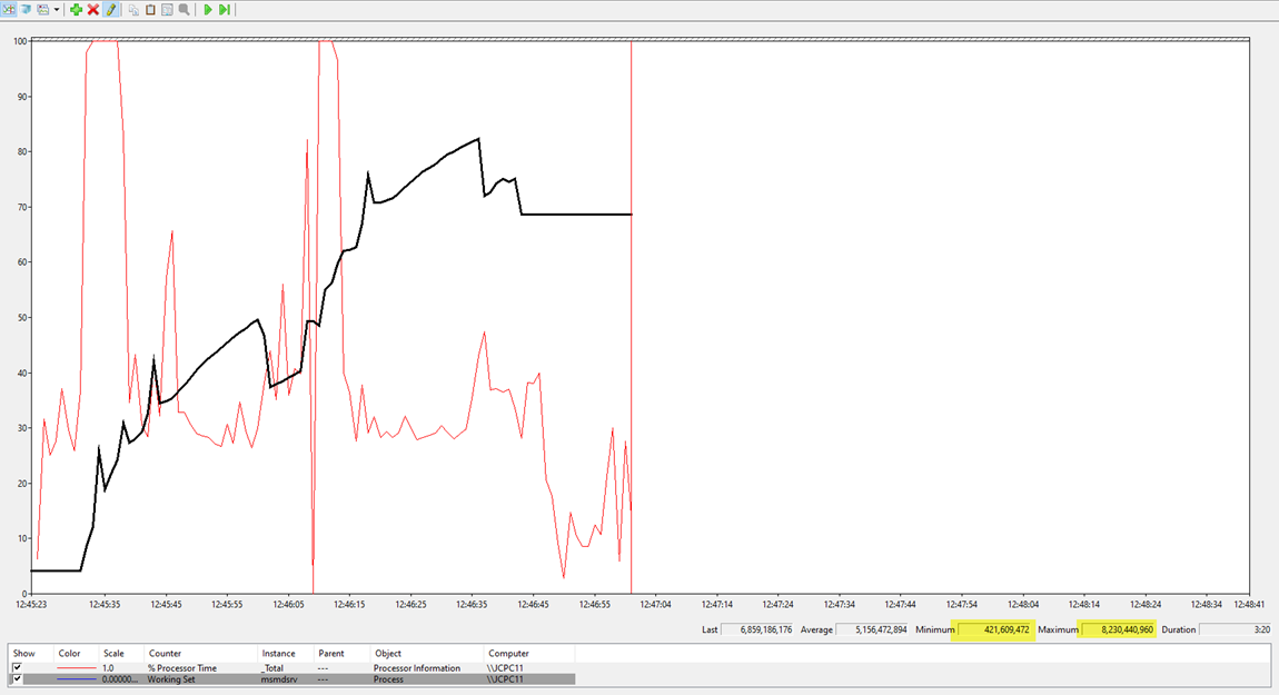
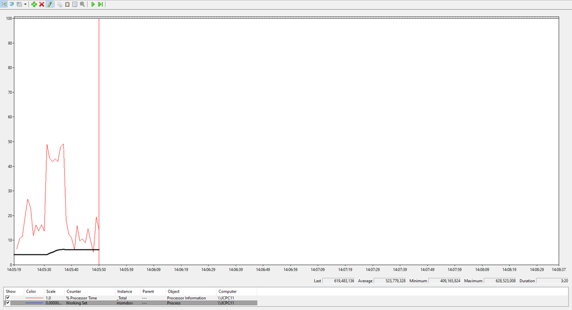
The following result took 71 seconds to complete on the dataset in PB desktop. And took almost 8GB of memory::
Memory profile during the DAX query:
If you try to publish this report to Power BI service, you will get the following message:
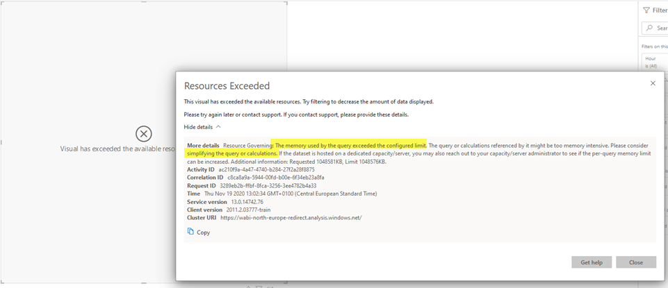
I was just WOW! But what can I tune on such a simple query and such a simple measure?
Tunning 1 – Rewrite Median?
I was a bit disappointed about the median function. When we used date for filtering, the performance of the query was ok. But when we used a larger dataset it was not performing at all.
I do know nothing about the inner implementation of the median function in DAX but based on memory consumption it seems like if there would be column materialization on the background and sorting when searching for the median.
Here’s a bit of theory about median and a bit of fact about columnar storage so we can discover how we can take advantage of the data combination/granularity we have in the model.
Below are two median samples for a couple of numbers – when the count of the numbers is Even and when is Odd. More median theory on Wikipedia.
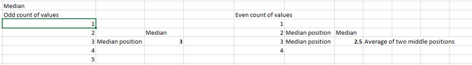
The rules for calculating median are the same, even when numbers in the set are repeating (non-unique). Here are the steps of the potential algorithm:
- Sort existing values.
- Find the median position(s).
- Take a value or two and make average to get median.
Let’s look at this from the perspective of column store where we have just a couple of values with hundreds of repeats.
As we know the count is very fast for column store and that could be our advantage as we have a small number of unique values repeated many times.
Following is an example of data where we can visualize the way how we can take advantage of the fact described above.
| Temperature |
Count |
Cumulative Count |
Cumulative Count Start |
| 12 |
500 |
500 |
1 |
| 13 |
500 |
1000 |
501 |
| 18 |
500 |
1500 |
1001 |
| 20 |
501 |
2001 |
1501 |
| Total Count |
2001 |
||
| Position of median Odd |
1001 |
||
| Position of median Even |
1001 |
In this case, we just need to go through 4 values and find in which interval our position of median belongs.
In the worst-case scenario, we will hit between two values like on the following picture (we changed the last count from 501 to 500):
| Temperature |
Count |
Cumulative Count |
Cumulative Count Start |
| 12 |
500 |
500 |
1 |
| 13 |
500 |
1000 |
501 |
| 18 |
500 |
1500 |
1001 |
| 20 |
500 |
2000 |
1501 |
| Total Count |
2000 |
||
| Position of median Odd |
1000 |
||
| Position of median Even |
1001 |
How to implement this in DAX:
First helper measures are count and cumulative count for temperature:
| MEASURE Senzors[RowCount] = COUNTROWS ( Senzors ) |
| MEASURE Senzors[TemperatureRowCountCumul] = VAR _curentTemp = MAX ( ‘Senzors'[temperature] ) RETURN CALCULATE ( COUNTROWS ( Senzors ), Senzors[temperature] <= _curentTemp ) |
Second and third measures give us a position of the median for given context:
| MEASURE Senzors[MedianPositionEven] = ROUNDUP ( ( COUNTROWS ( Senzors ) / 2 ), 0 ) |
| MEASURE Senzors[MedianPositionOdd] = VAR _cnt = COUNTROWS ( Senzors ) RETURN ROUNDUP ( ( _cnt / 2 ), 0 ) — this is a trick where boolean is auto-casted to int (0 or 1) + ISEVEN ( _cnt ) |
The fourth measure – Calculated median – does what we described in the tables above. Iterate through temperature values and find rows that contain median positions and make average on that row(s).
| MEASURE Senzors[Calc_Med] = — get two possible position of median VAR _mpe = [MedianPositionEven] VAR _mpeOdd = [MedianPositionOdd] — Make Temperature table in current context with Positions where value starts and finishes VAR _TempMedianTable = ADDCOLUMNS ( VALUES ( Senzors[temperature] ), “MMIN”, [TemperatureRowCountCumul] – [RowCount] + 1, “MMAX”, [TemperatureRowCountCumul] ) — Filter table to keep only values which contains Median positions in it VAR _T_MedianVals = FILTER ( _TempMedianTable, (_mpe >= [MMIN] && _mpe <= [MMAX] ) || (_mpeOdd >= [MMIN] && _mpeOdd <= [MMAX] ) ) — return average of filtered dataset (one or two rows) RETURN AVERAGEX ( _T_MedianVals, [temperature] ) |
Maximum number of rows which goes to the final average is 2.
Let us see the performance of such measure:
| Performance for Hour (24 values) | Duration (s) | Memory Consumed (GB) |
| Native median function |
71 |
8 |
| Custom implementation |
6.3 |
0.2 |
Sounds reasonable and promising!
But not so fast – when the number of values by which we group the data grow, the duration grows as well.
Here are some statistics when removing hour (24 values) and bringing location (400+ values) into the table.
| Performance for location (422 values) | Duration (s) | Memory Consumed (GB) |
| Native Median Function |
81 |
8 |
| Custom Implementation |
107 |
2.5 |
Look at the memory consumption profile of calculated median for location below:
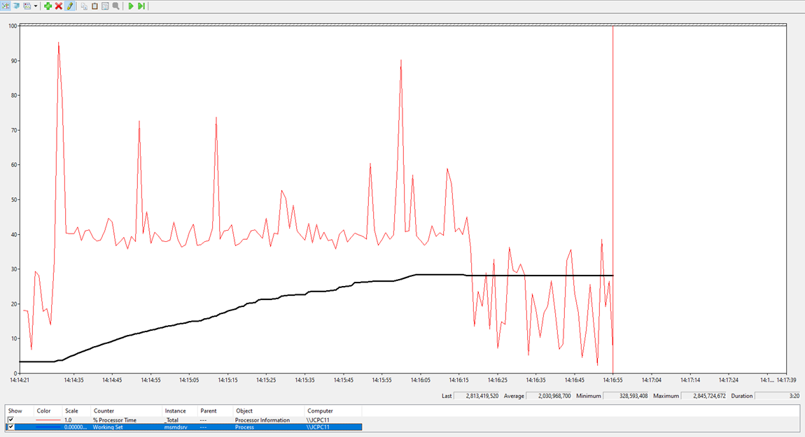
That is not so good anymore!
Our custom implementation is a bit slower for location and despite the fact it is consuming a lot less memory, this will not work in Power BI service as well.
This means that we solved just a part of the puzzle – our implementation is working fine only when we have a small number of values that we are grouping by.
So, what are the remaining questions to make this report working in PBI service?
- How to improve the overall duration of the query?
- How to decrease memory consumption?
Tuning 2 – Reduce Memory Consumption
We start with the memory consumption part. First, we need to identify which part of the formula is eating so much memory.
Actually, it is the same one that has the most performance impact on the query.
It’s this formula for the cumulative count, which is evaluated for each row of location multiplied by each value of temperature:
| MEASURE Senzors[TemperatureRowCountCumul] = VAR _curentTemp = MAX ( ‘Senzors'[temperature] ) RETURN CALCULATE ( COUNTROWS ( Senzors ), Senzors[temperature] <= _curentTemp ) |
Is there a different way to get a cumulative count without using CALCULATE? Maybe a more transparent way for the PB engine? Yes, there is! We can remodel the temperature column and define the cumulative sorted approach as a many-to-many relationship towards the sensors.
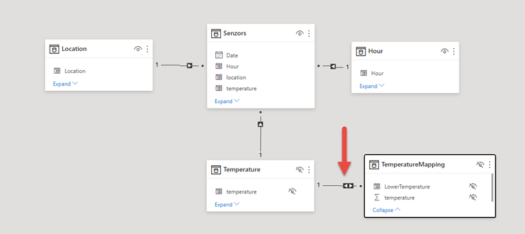
Sample content of temperature tables would look like this:
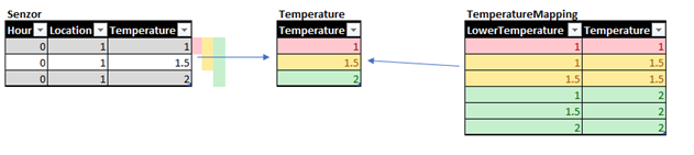
I believe that the picture above is self-describing.
As a result of this model, when you use the temperature attribute from the TemperatureMapping table, you have:
– Cumulative behavior of RowCount.
– Relation calculated in advance.
For this new model version, we define measures as below:
RowCount measure we have already, but with temperature from Mapping table, it will give us CumulativeCount in fact.
| MEASURE Senzors[RowCount] = COUNTROWS ( Senzors ) |
We must create a new measure which will give us a normal count for the mapping table to be able to calculate the starting position of the temperature value:
| MEASURE Senzors[TemperatureMappingRowCount] = CALCULATE ( [RowCount], FILTER ( TemperatureMapping, TemperatureMapping[LowerTemperature] = TemperatureMapping[temperature] ) ) |
New median definition:
| MEASURE Senzors[Calc_MedTempMap] = VAR _mpe = [MedianPositionEven] VAR _mpeOdd = [MedianPositionOdd] VAR _TempMedianTable = ADDCOLUMNS ( VALUES ( TemperatureMapping[temperature] ), “MMIN”, [RowCount] – [TemperatureMappingRowCount] + 1, “MMAX”, [RowCount] ) VAR _T_MedianVals = FILTER ( _TempMedianTable, (_mpe >= [MMIN] && _mpe <= [MMAX] ) || (_mpeOdd >= [MMIN] && _mpeOdd <= [MMAX] ) ) RETURN AVERAGEX ( _T_MedianVals, [temperature] ) |
Alright, let’s check the performance – the memory consumption is now just in MBs!
| Performance Many2Many Median | Duration (s) | Memory Consumed (GB) |
| Used with Hours |
2.2 |
0,02 |
| Used with location |
41.1 |
0,08 |
I think we can be happy about it and the memory puzzle seems to be solved.
You can download a sample PBI file (I decreased data to only one month of the data, but you can download the whole dataset).
Below is the statistics summary for now:
| Performance for Hour (24 values) | Duration (s) | Memory Consumed (GB) |
| Native median function |
71.00 |
8.00 |
| Custom implementation |
6.30 |
0.20 |
| Many2Many median |
2.20 |
0.02 |
| Performance for Location (422 values) | Duration (s) | Memory Consumed (GB) |
| Native median function |
81.00 |
8.00 |
| Custom implementation 1 |
107.00 |
2.50 |
| Many2Many median |
41.10 |
0.08 |
I’ll stop this blog here, as it is too long already. Next week, I’ll bring the second part in regards to how to improve performance, so the user has a better experience while using this report.


1 Comment. Leave new
[…] my last blog post, I have addressed an issue with DAX Median function consuming a lot of memory. To refresh the […]